Home - Sokheng Din

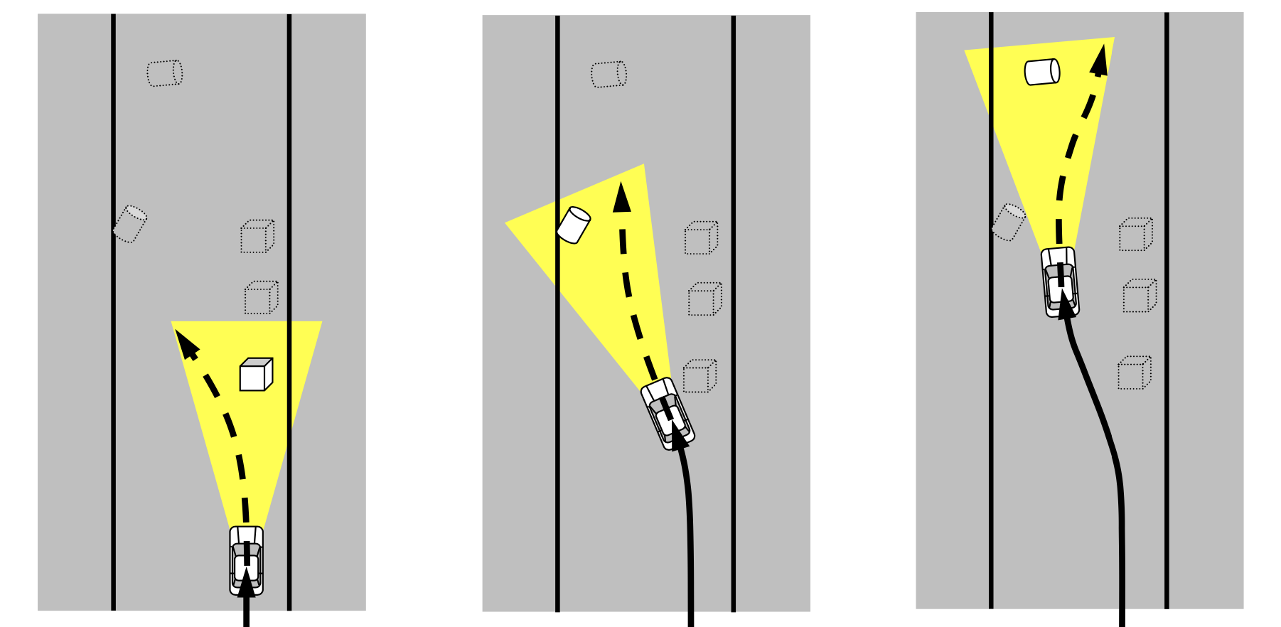
What is Model Predictive Control ?

Model Predictive Control (MPC) is the optimal control method that use optimization algorithms to solve the cost function the occurs from the desired input and obtain back the optimal input control over the finite and infinite horizons. Recently, MPC is hyping up among the control system researcher, since it is fast, efficiency and robustness for any high complex system.

A car with finite horizons prediction and set point prediction over finite horizons.

Nonlinear Model Predictive Control ?

Nonlinear Model Predictive Control has the same basic core of its control algorithms. The different is about the mathematical solving over the system.
In the real-life application, most of the system certainly nonlinear and it's more complex than linear model. Linear systems are mostly time-invariant, meaning that the response of the system input is time-independent. Nonlinear systems are time-varying meaning that the response of the system to any input is time-dependent.

The system model can be represent as state-space model

$$ \dot{X} = f(X,U) $$

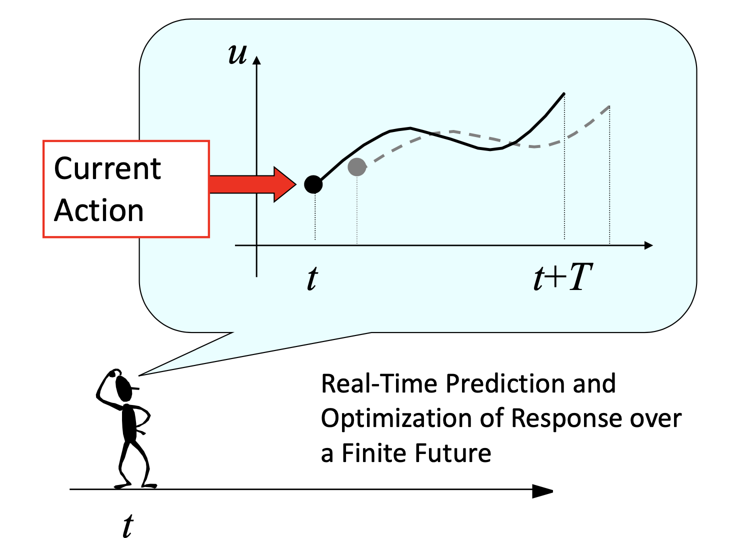
Nonlinear Model Predictive Control also works by solving the quardratic cost subject to the nonlinear function over a future finite horizons. The quadractic cost can be define as

J(x,u) = \displaystyle\sum_{k=0}^{N-1}(X_{k, ref}-X_{k})^{T}Q(X_{k, ref}-X_{k})+(U_{k,ref}-U_{k})^{T}R(U_{k,ref}-U_{k}) + \phi(X_{N})

Notation

$X$
is the state of the system. This shall be obtained from the optimiztion problem.
$X_{ref}$
is the reference state of the system or desired input state.
$U$
is the input control of the system. This is a solution obtained from the optimization problem.
$U_{ref}$
is the reference control of the system or desired input control.

Rewrite the optimization of NMPC problem.

\begin{align*} \min_{u_{0}, u_{1}, ..., u_{N-1} } \quad \sum_{k=0}^{N-1}(X_{k, ref}-X_{k})^{T}&Q(X_{k, ref}-X_{k})+(U_{k,ref}-U_{k})^{T}R(U_{k,ref}-U_{k}) + \phi(X_{N})\\ \text{subject to} \quad & x_{k+1} = f(x_k, u_k) \quad \text{(System dynamics)} \\ & g(x_k, x_k) \leq 0 \quad \text{(State constraints)} \\ & h(x_k, x_k) \leq 0 \quad \text{(Input constraints)} \\ & p(x_k) \leq 0 \quad \text{(Path constraints)} \\ & x_0=x(0) \quad \text{(Initial condition)} \end{align*}

Which,

$f$
is the system dynamics model.
$g$
is the state constraints of the system.
$h$
is the input constraints of the system.
$p$
is the path constraint, it help to ensure the safety following path of our system.
$\phi(X_{N})$
is the terminal cost of the system.

Discretize the system model with Runge-Kutta 4th order

I will choose a simple system mode robot DifferentialDrive . The forward kinematic equation

\begin{bmatrix} v_{x} \\ v_{y} \\ v_{\theta} \end{bmatrix} = \begin{bmatrix} v\sin{(\theta)} \\ v\cos{(\theta)} \\ \omega \end{bmatrix}

State constraints are the restriction imposed on the state variable of the system. It helps our optimizer not to obtain the solution that is outside the boundary region and also ensure the system to always perform the minimal action control in any critical condition.

We, then can do the approximation

\begin{align*} k_{1} &= f(x^{*}, u^{*}) \\ k_{2} &= f(x^{*}+k_{1}\frac{dt}{2}, u^{*}) \\ k_{3} &= f(x^{*}+k_{2}\frac{dt}{2}, u^{*}) \\ k_{4} &= f(x^{*}+k_{3}dt, u^{*}) \\ \Rightarrow{x_{k+1} } &= x_{k} + (k_{1}+2k_{2}+2k_{3}+k_{4})\frac{dt}{6} \end{align*}

Let's evaluate it with our model.

\begin{align*} k_{1} &= \begin{bmatrix} v^{*}\cos{(\theta)} \\ v^{*}\sin{(\theta)} \\ \omega^{*} \end{bmatrix} \\ k_{2} &= \begin{bmatrix} v^{*}\cos{(\theta + \frac{dt}{2} \times k_{1})} \\ v^{*}\sin{(\theta+ \frac{dt}{2}\times k_{1})} \\ \omega^{*} \end{bmatrix} \\ k_{3} &= \begin{bmatrix} v^{*}\cos{(\theta + \frac{dt}{2} \times k_{2})} \\ v^{*}\sin{(\theta+ \frac{dt}{2}\times k_{2})} \\ \omega^{*} \end{bmatrix} \\ k_{4} &= \begin{bmatrix} v^{*}\cos{(\theta + dt \times k_{3})} \\ v^{*}\sin{(\theta+ dt\times k_{3})} \\ \omega^{*} \end{bmatrix} \\ \end{align*}

\Rightarrow{x_{k+1} } = x_{k} + \left( \begin{bmatrix} v^{*}\cos{(\theta)} \\ v^{*}\sin{(\theta)} \\ \omega^{*} \end{bmatrix} + 2 \times \begin{bmatrix} v^{*}\cos{(\theta + \frac{dt}{2} \times k_{1})} \\ v^{*}\sin{(\theta+ \frac{dt}{2}\times k_{1})} \\ \omega^{*} \end{bmatrix} + 2 \times \begin{bmatrix} v^{*}\cos{(\theta + \frac{dt}{2} \times k_{2})} \\ v^{*}\sin{(\theta+ \frac{dt}{2}\times k_{2})} \\ \omega^{*} \end{bmatrix} + \begin{bmatrix} v^{*}\cos{(\theta + dt \times k_{3})} \\ v^{*}\sin{(\theta+ dt\times k_{3})} \\ \omega^{*} \end{bmatrix} \right) \frac{dt}{6}

How to implement it in Python ???

import numpy as np

## Define sampling time dt 100Hz
dt = 0.01
## Define the num steps for function approximation 
num_steps = 100
## Define initial states
x = 0.0
y = 0.0
yaw = 0.0
## Define input control
v = 1.5 #m/s
omega = 1.57 #rad/s
## Define state represent model
### define lambda function take variable x
f = lambda x, u :  np.array([
      [u[0]*np.cos(x[2])],
      [u[0]*np.sin(x[2])],
      [u[1]]
])

for _ in range(num_steps):
    k1 = f([x, y, yaw], [v, omega])
    k2 = f([x + (dt / 2) * k1[0], y + (dt / 2) * k1[1], yaw + (dt / 2) * k1[2]], [v, omega])
    k3 = f([x + (dt / 2) * k2[0], y + (dt / 2) * k2[1], yaw + (dt / 2) * k2[2]], [v, omega])
    k4 = f([x + dt * k3[0], y + dt * k3[1], yaw + dt * k3[2]], [v, omega])

    # Update state of the robot
    x += (k1[0] + 2 * k2[0] + 2 * k3[0] + k4[0]) * dt / 6
    y += (k1[1] + 2 * k2[1] + 2 * k3[1] + k4[1]) * dt / 6
    yaw += (k1[2] + 2 * k2[2] + 2 * k3[2] + k4[2]) * dt / 6

Single Shooting Method

Single Shooting Method is a method that we transform the optimal control problem to the nonlinear programming problem with just one decision variable.

\begin{align*} \text{Problem Decision Variable} \\ w = \left [ u_{0}, ..., u_{N-1}\right] \end{align*}

\begin{align*} x_{u} &= F(w,x_{0},t_{k}) \\ F(w,x_{0},t_{0}) &= x_{0} \\ \end{align*}

Then solve the NLP

\begin{align*} \min_{w}\Phi(F(w,x_{0},t_{k}), w) \\ \text{Subject to} \hspace{1cm} g_{1}(F(w,x_{0},t_{k}),w) \leq{0} \end{align*}

Multiple Shooting Method

Multiple Shooting Method is a method that consist of transforming of optimal control problem to the nonlinear programming problem with multiple decision variables.

\begin{align*} \text{Problem Decision Variable} \\ w = \left [ u_{0}, ..., u_{N-1}, x_{0}, ..., x_{N}\right] \end{align*}

$X$
becoming decision variable in the opimization problem as well as u
We apply path constraint at each iteration step

\begin{equation*} x_{k+1}-f(x_{k},u_{k}) = 0 \end{equation*}

Then solve the NLP

\begin{align*} \min_{w} \Phi(F(w,x_{0},t_{k}),& w) \\ \text{s.t}\hspace{0.5cm} g_{1}(F(w,x_{0},t_{k}),w) &\leq{0} \\ g_{2}(w) = \begin{bmatrix} \bar{x}_{0}-x_{0} \\ f(x_{0},u_{0})-x_{1} \\ \vdots \\ f(x_{N-1}, u_{N-1}-x_{N}) \end{bmatrix} &= 0 \end{align*}

Full Implement in Python

We will use Casadi as a numerical optimization framework.

import casadi as ca

Define state representation and input control of our nonlinear model.

# Symbolic Variables
## States
x = ca.SX.sym("x")
y = ca.SX.sym("y")
theta = ca.SX.sym("theta")
states = ca.vertcat(x, y, theta)
num_states = states.numel()

## Control
u1 = ca.SX.sym("u1")
u2 = ca.SX.sym("u2")
controls = ca.vertcat(u1, u2)
num_controls = controls.numel()

# Define Nonlinear model
## Rotation Matrix
rot_mat = ca.vertcat(
    ca.horzcat(ca.cos(theta), ca.sin(theta), 0),
    ca.horzcat(-ca.sin(theta), ca.cos(theta), 0),
    ca.horzcat(0, 0, 1)
)

vx = u1 * ca.cos(theta)
vy = u1 * ca.sin(theta)
vyaw = u2

rhs = ca.vertcat(vx, vy, vyaw)
## Define mapped nonlinear function f(x,u) -> rhs
f = ca.Function('f', [states, controls], [rhs])

Declare symbolic matrix

X = ca.SX.sym('X', num_states, prediction_horizons + 1)
X_ref = ca.SX.sym('X_ref', num_states, prediction_horizons + 1)
U = ca.SX.sym('U', num_controls, prediction_horizons)
U_ref = ca.SX.sym('U_ref', num_controls, prediction_horizons)

Define nonlinear programming and options for Casadi

nlp_prob = {
    'f': cost_fn,
    'x': opt_var,
    'p': opt_dec,
    'g': g
}

nlp_opts = {
    'ipopt.max_iter': 5000,
    'ipopt.print_level': 0,
    'ipopt.acceptable_tol': 1e-6,
    'ipopt.acceptable_obj_change_tol': 1e-4,
    'print_time': 0
}

Determine boundary and constraint for our optimizer

lbx = ca.DM.zeros((num_states * (prediction_horizons + 1) + num_controls * prediction_horizons, 1))
ubx = ca.DM.zeros((num_states * (prediction_horizons + 1) + num_controls * prediction_horizons, 1))

lbx[0: num_states * (prediction_horizons + 1): num_states] = x_min
lbx[1: num_states * (prediction_horizons + 1): num_states] = y_min
lbx[2: num_states * (prediction_horizons + 1): num_states] = theta_min

ubx[0: num_states * (prediction_horizons + 1): num_states] = x_max
ubx[1: num_states * (prediction_horizons + 1): num_states] = y_max
ubx[2: num_states * (prediction_horizons + 1): num_states] = theta_max

lbx[num_states * (prediction_horizons + 1): num_states * (prediction_horizons + 1) + num_controls * prediction_horizons: num_controls] = u_min
lbx[num_states * (prediction_horizons + 1) + 1: num_states * (prediction_horizons + 1) + num_controls * prediction_horizons: num_controls] = u_min

ubx[num_states * (prediction_horizons + 1): num_states * (prediction_horizons + 1) + num_controls * prediction_horizons: num_controls] = u_max
ubx[num_states * (prediction_horizons + 1) + 1: num_states * (prediction_horizons + 1) + num_controls * prediction_horizons: num_controls] = u_max

args = {
    'lbg': ca.DM.zeros((num_states * (prediction_horizons + 1), 1)),
    'ubg': ca.DM.zeros((num_states * (prediction_horizons + 1), 1)),
    'lbx': lbx,
    'ubx': ubx
}

Obtain the solution from the solver at each iteration

sol = solver(
            x0=args['x0'],
            p=args['p'],
            lbx=args['lbx'],
            ubx=args['ubx'],
            lbg=args['lbg'],
            ubg=args['ubg'],
        )

        sol_x = ca.reshape(sol['x'][:num_states * (prediction_horizons + 1)], 3, prediction_horizons + 1)
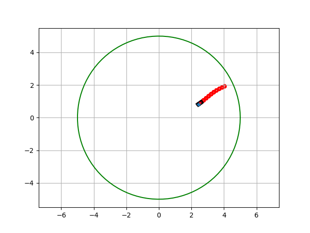
        sol_u = ca.reshape(sol['x'][num_states * (prediction_horizons + 1):], 2, prediction_horizons)

Result

I use MPC to control the differential drive robot to move from it zero position the the desired postion that I want to follow !. I generate a circle trajectory and I fit this curve into my beautiful and robustness cost and then volia !!!.

Plot of differential drive robot follow the circle trajectory !!!.

In conclusion

In my opinion, I think MPC is suitable for the control system, since it can provide the significant control input that was predicted over the finite future of time. This can ensure the safety of the system and also can provide a quick look or reaction to the control action of the system too.

Nonlinear Model Predictive Control

Author: Din Sokheng