Introduction to PID Controller in Python

What is PID Controller ?

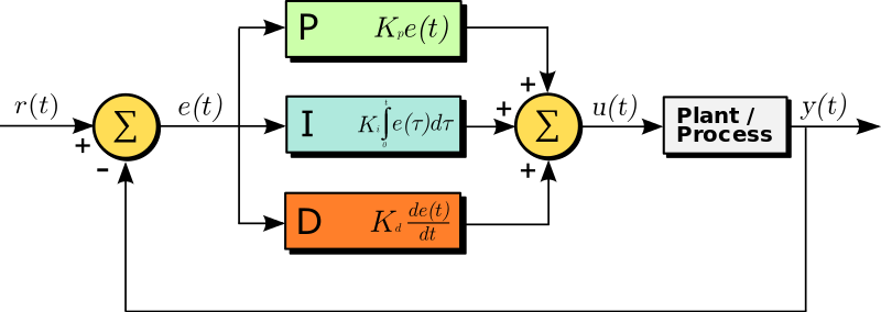
The Proportional Integral Derivative (PID) controller is a traditional method in control systems that has found widespread use in control system engineering and industrial applications since its emergence in the 1940s. A PID controller is considered a feedback controller, aiming to minimize the error between the system's feedback and the desired setpoint by manually or automatically fine-tuning the coefficients

.

How it works ?

Imagine you want to control the speed of a DC motor to reach 300 RPM, but due to the natural response of the DC motor, it cannot reach the desired angular speed. PID offers a solution to this natural response by adjusting the system's time response using its three components, as shown in the formula below.

Formulation

• $K_{P}$
  represents the proportional gain.
• $K_{I}$
  represents the integral gain.
• $K_{D}$
  represents the derivative gain.
• $e(t)=target-feedback$
  is the error between target point and feedback of the system

Response Time

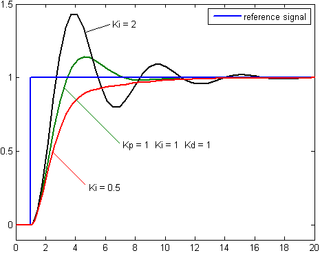
As you can see in the figure above, the response time of the system is difference.

• The response time with
  $K_{I}=2$
  the system is likely to overshoot before reaching the steady-state, which may not be suitable for applications like controlling a DC motor.
• The response time with
  $K_{i}=0.5,$
  the response does not overshoot but has a slower response to reach the steady-state.
• The response time with
  $K_{p}=1, K_{i}=1, K_{d}=1$
  there is a slight overshoot, but the steady-state is reached faster.

How can we write PID code in Python ?

Let's use a differential drive robot as a case study system. A differential drive robot is commonly used in robotics and automation, making it an ideal choice for a demonstration.

The configuration of Differential Drive Robot in axes OXY.

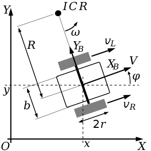
The forward kinematic equation

So, if we discretize the forward kinematic with a certain sampling time, we will get

In Python,

class DifferentialDrive:
    def __init__(self):
        self.r = 0.05
        self.L = 0.25
    def forward_kinematic(self, v, omega, yaw):
        vx = v*np.cos(yaw)
        vy = v*np.sin(yaw)
        vyaw = omega

        return vx, vy, vyaw
    def discrete_state(self, x, y, yaw, v, omega, dt):
        dx, dy, dyaw = self.forward_kinematic(v, omega, yaw)
        x_next = x + dx * dt
        y_next = y + dy * dt
        yaw_next = yaw + dyaw * dt

        return x_next, y_next, yaw_next

The DifferentialDrive class that we defined, has all the need attribute to use for PID control !!. We just need to write another class for our PID Controller .

class PIDController:
    def __init__(self, kp, ki, kd, dt):

        self.kp = kp
        self.ki = ki
        self.kd = kd
        self.dt = dt
        self.integral = 0

    def calculate_pid(self, errors):
        # Calculate proportional error
        proportional = self.kp * errors[-1]
        # Calculate integration error
        integral = self.integral + self.ki * (errors[-1]) * self.dt
        self.integral = integral
        # Calculate derivative error
        derivative = self.kd * (errors[-1] - errors[-2])/self.dt

        output = proportional + integral + derivative

        return output

Don't worry, this class just defined as the PID formula. So, by doing this, we will be able to use all the characteristic of our PID controller.

Experiment

PID for point control

If I want my DifferentialDrive robot go to point

, Then I can calculate the error between the reference point and the feedback position of the robot. I simulated my robot in the for loop and calculate this error recursively.

error_x.append(ref_path[0]-current_x)
error_y.append(ref_path[1]-current_y)
error_yaw.append(ref_path[2]-current_yaw)

Then, let's apply PID

output_vx = pid_controller_x.calculate_pid(error_x)
output_vy = pid_controller_y.calculate_pid(error_y)
output_omega = pid_controller_yaw.calculate_pid(error_yaw)

We will also need to update current position of the robot with the given optimal value from the PID controller.

x_next, y_next, yaw_next = diff_drive.discrete_state(current_x, current_y, current_yaw, v_pid, omega_pid, sampling_time) # Skip for omega we only look for x, y
current_x = x_next
current_y = y_next
current_yaw = yaw_next

I use matplotlib library to simulate my robot.

plt.clf()
plt.gcf().canvas.mpl_connect('key_release_event',
            lambda event: [exit(0) if event.key == 'escape' else None])
plot_arrow(current_x, current_y, current_yaw)
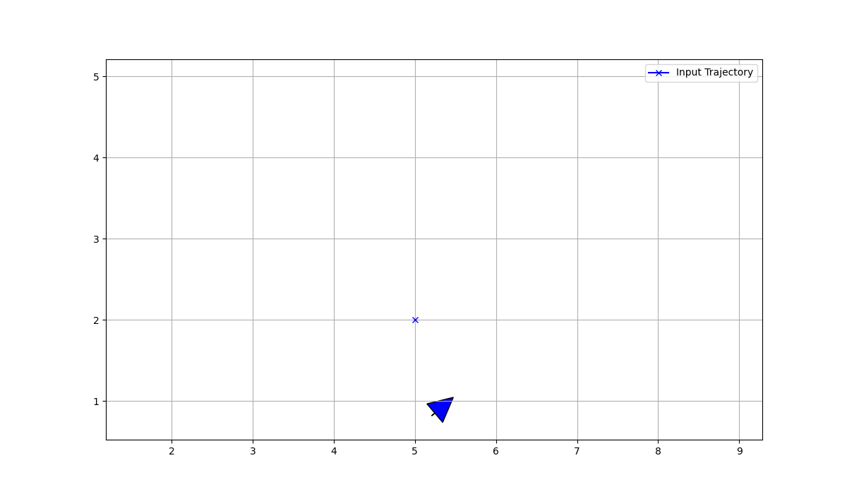
plt.plot(5, 5)
plt.plot(ref_path[0], ref_path[1], marker="x", color="blue", label="Input Trajectory")
plt.axis("equal")
plt.grid(True)
plt.legend()
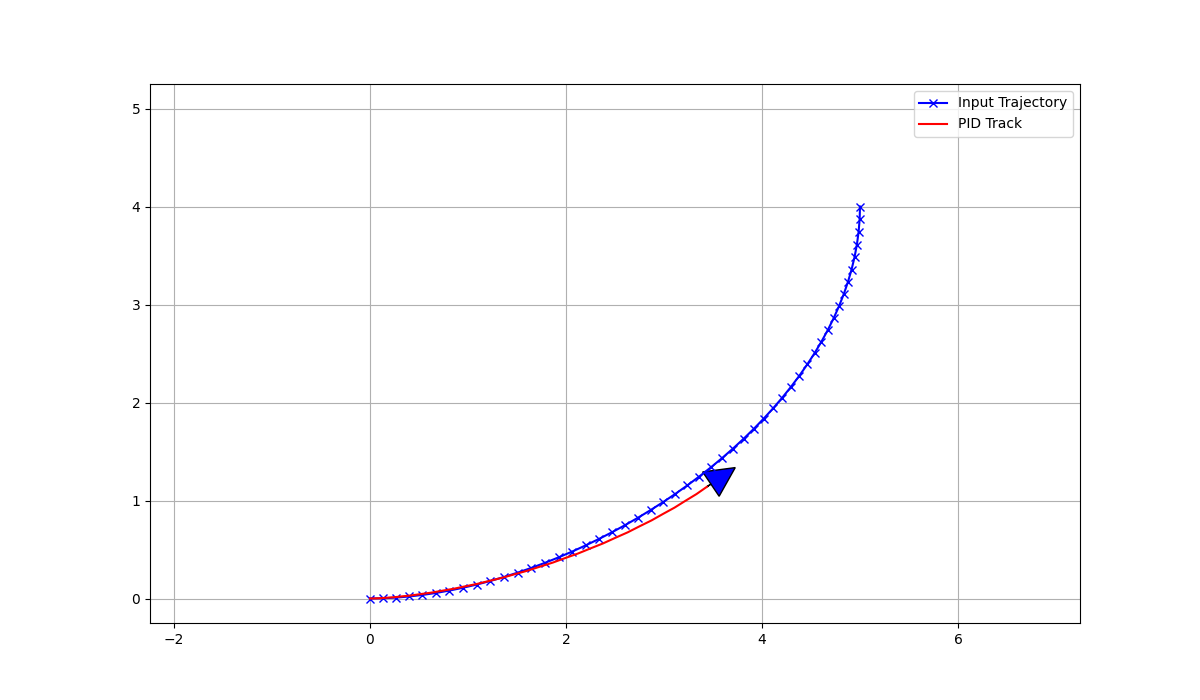
plt.pause(0.0001)

Path Tracking

The code is all way the same. The different is that, I fit the continuous point into the robot instead of fixed goal point. I use BeizerCurve function to generate Spline Trajectory for the robot.

The full code is published open-source on my Github. Link here Github. Hit the star for me if you like my work 🙂.

Result

In Conclusion

In my opinion, the PID Controller is an excellent choice for most control system applications due to its simplicity and powerful capabilities in handling complex control challenges arising from various systems.

References

1. BeizerCurve
2. PID Controller: Control Systems Engineering by Normal S. Nise.
3. Beizer Path
4. PID Lecture